Those of us who are into neural networks and deep learning, most probably have heard this: Training neural networks is like doing both art & magic at the same time. The fact is this statement seems to hold true in many cases, but there is math & science behind the shining magic, which can be mastered of course. I believe anyone interested in the topic should also be motivated to dig deeper into this wonderland after knowing that there are plenty of artistic maneuvers to be taken.

Before you continue: I assume that the reader is already familiar with the basic terminologies involved in machine learning, deep learning and neural networks. I’ve tried to keep things as simple as it can be, so hopefully it’ll be helpful for anyone, regardless of their level of expertise.

Also, I should mention that majority of what you’ll read is backed up by fair amount of code, which I’m planning to update soon and add the link here. Most of the code is already written and tested. Gladly, only a few more tests remain (it involves heavy GPU computations).

Ok, enough for introduction I think, since we have so much to cover. Let’s go ahead starting with important hyperparameters in deep learning.

Batch Size & Learning Rate

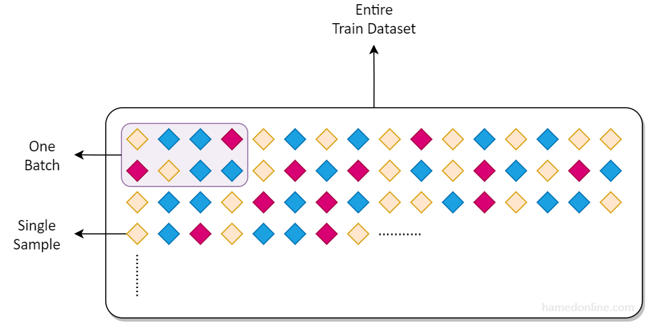
Batch size refers to the number of samples that is propagated through neural network in each weight parameters adjustment iteration. The more samples we pass in during each iteration, the less steps are needed to complete one epoch (an epoch means one full propagation of the entire training data through the network). This implies that the larger the batch size gets, the quicker the network weights get updated. But, there’s a caveat.

The popular view among deep learning community is that larger batch sizes don't help if you want your model to generalize well. More samples in each observation results in sacrificing attention to details and regularization effect of proper noise, compared to when smaller bunches of data are used for each learning iteration. In fact, one of the downsides of using large batch sizes is that it might lead to solutions that generalize worse than those trained with smaller batches. But is this always true? And if so, are there any ways to mitigate the side effects? We’ll see that in a moment, after reviewing the concept of learning rate.

So what is the learning rate? In simple terms, it specifies how much we would like the weights of network to be adjusted in each iteration of learning (weight adjustment gets done after calculating loss for each batch). In another prospective, LR determines the length of steps towards the hopefully global minima in loss space.

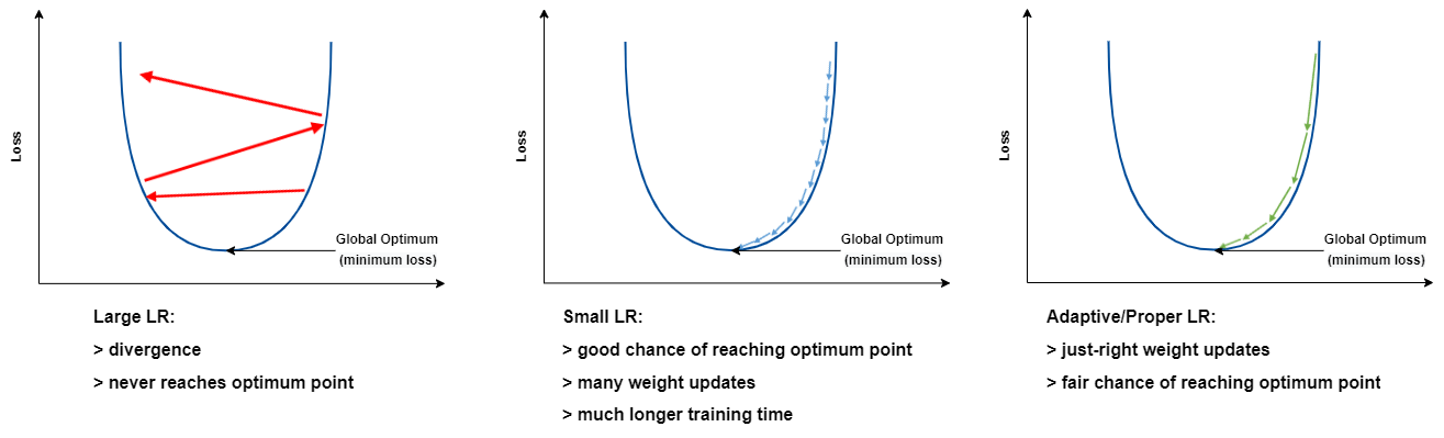
You might’ve already seen a similar plot to below one that demonstrates the step size in each iteration to reach the optimal point. This step size is determined by learning rate. Too large LR results in divergence and too small LR prolongs training time.

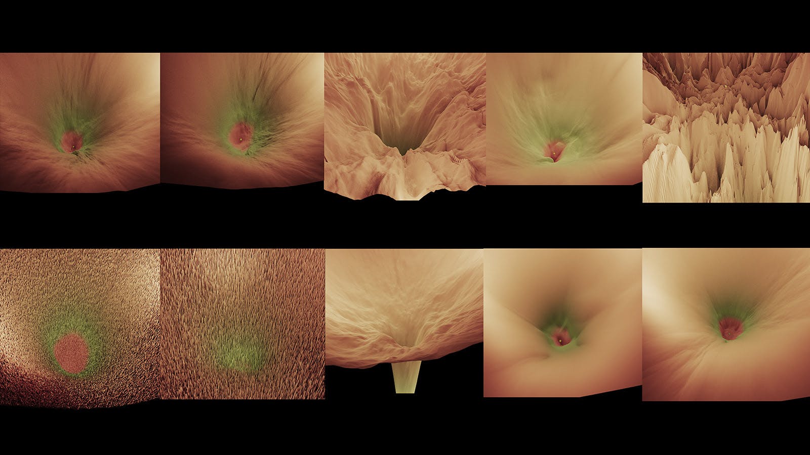
The loss landscape looks like a scenery with hills, mountains and valleys. The optimal point in this landscape is the deepest valley point in the global loss space, with the lowest loss value. The area highlighted in red in following images refers to optimal loss.

There is no universal good learning rate that works well for all datasets. Picking an optimal learning rate depends on the topology of the loss landscape, which itself is a result of the dataset, batch size and model architecture (even the activation functions used in model architecture affects the loss landscape). As you can see from above picture, there could be multiple local minima loss points, depending on our dataset. That’s why it is advised broadly to use learning rate schedulers, which change the learning rate during training time, in order to avoid getting stuck at a local minima.

Now that the picture is less blurry to our eyes, we can kind of understand why "learning rate" and "batch size" together are probably the most impactful factor we need to look for when training neural networks, as they have been proven to be interrelated in the mechanism of neural networks training.

Daryl Chang and Apurva Pathak have experimented and written up an excellent post describing the relationship details between batch size & learning rate, while discussing their effect on model training extensively (highly recommended read if you're interested). Their results show that careful relative tuning of both the batch size and learning rate can achieve competitive performance, and it comes with a huge advantage of course: faster training.

The article’s takeaway for us? We'd better use linear scaling rule. When the batch size is multiplied by k, we'd better also multiply the learning rate by k.

In other words, we shouldn't play with batch size hyperparameter blindly, while keeping the learning rate fixed.

Choosing a Proper Batch Size

There are couple of points we need to take into account when choosing the batch size according to the things discussed so far.

• As the batch size grows, it becomes easier for our model to overfit the data (less generalization). We need to increase the learning rate in linear fashion to alleviate this effect.
• Hardware capabilities for batch computation is important. We can only increase batch size up to GPU or TPU memory limit we’re provided with.

Ok. Suppose you run a test and notice that 16 images per iteration is the batch size limit you cannot cross, and you get “GPU ran out of memory” errors above that. Is this a good size to go along with? As far as training speed goes, this size would give us the fastest training possible by current machine we have at our disposal. So far so good. Should we jump on training then? My answer is no. There’s something else I consider before finalizing this value. Let me explain it by an example.

Imagine you’re a librarian with no domain knowledge around books! You don’t know the book categories and have no idea how to group them, by looking only at their cover and title. You’re given a training session that contains batch of books on a desk (with limited room on it), and hopefully each sample book has a label so that you can learn how the title and covers could indicate which category each book belongs to. If you continue to see multiple batches in your training sessions, you should start to learn from examples laid out for training. What matters is that you’re shown decent amount of samples in each step, and there better be enough samples from every class in each batch so that you can pay attention to the differences that makes it easier to distinguish one from another.

Now, just like not having a sample of a class in each batch, too many samples for each class per step might not be wise too, unless you’re a fast learner with higher learning rate. You might miss some little details here and there though when you’re learning faster. You get the idea?

In my humble opinion, number of classes or category size is another deciding factor to consider when reaching a conclusion on batch size. With a supposedly balanced dataset, I always like to see at least 2 or 3 samples of each class passed to every iteration batch. So, if you have for example 5 target classes in your dataset, 16 looks like a good number for batch size (5x3=15). I wouldn’t say the same for a classification problem with 35 categories. 16 samples per batch falls short for such a dataset.

To summarize: In a classification problem, choose the batch size according to the number of classes and hardware capabilities. Larger batch sizes do train faster, but you need a proper learning rate to compensate for less generalization they come with.

Finding a Good Learning Rate

Now that we’ve decided the batch size, we need to look for a good learning rate. One neat tool for PyTorch is "PyTorch learning rate finder". You can also check this detailed post about implementation of an equivalent tool for Keras.

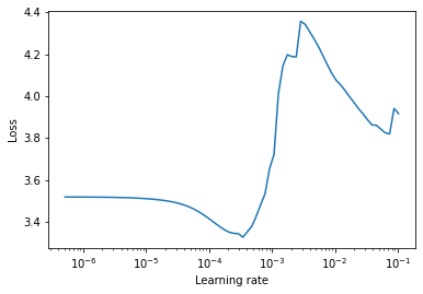
According to the documentation, the main idea here is that “a good static learning rate can be found half-way on the descending loss curve”. Therefor we can perform another LR search and take a more zoomed-in look at the range of learning rate that loss declines in above plot:

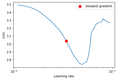
This tool can be utilized to find a LR that has the steepest gradient. The suggestion should be enough for us in order to begin further discoveries around that number.

Combination of a good learning rate with schedulers that modify it during training, can do wonders for a great training. There are great articles about LR schedulers out there and I won’t get into that subject.

Model Architecture

The model architecture itself can be regarded as an important independent parameter. It is investigatable in two aspects:

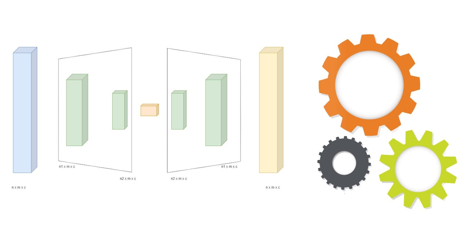
• The backbone we use to extract low dimensional space features (or embeddings) from input vectors. As an example, we can mention BERT language model for Natural Language Processing and ResNet50 Convolutional Neural Network for Image Processing.
• The final hidden layer(s) of the whole model architecture for fine-tuning (number of hidden layers, number of neurons in each layer, activation function type, etc.).

Backbone

Choosing a backbone depends on problem domain, context and complexity. We should also consider inference speed for production purposes when selecting a right fit. Bear in mind that if you want to compare multiple different backbones, the global loss space changes when swapping backbone and therefore all the tuning subjects must be reinitialized and done from the beginning for the new configuration.

Fine-tuning Layer(s)

The last hidden layer(s) and the corresponding hyperparameters we want to tune and decide on, can be investigated further as we settle on a particular backbone. Most of the time, I define a dictionary holding values for different setups and pass it into the loop that looks for model training and scoring based on those specific values. An example is as follows.

tune_subject = 'Number of Hidden Units'
tune_values = [64, 128, 256, 512, 1024]

for value in tune_values:
    print(f'Starting Training for {tune_subject}: {value}')
    ....
    nn_options_dict_step = {
        'n_hidden_layers': 1,
        'n_hidden_units': value,
        'use_dropout': False,
        'dropout_val': 0.2,
        'use_activation_fn': True,
        'activation_fn': nn.ReLU()
    }
    ....

As the code suggests, the different subjects of study can be easily defined and looked upon in this way, based on our needs. Again, the priority for us should be starting with the values that can make the biggest difference.

The last note that I would like to mention here is that as one goes further down this road, he/she should put aside a great deal of time studying deeper into the philosophy and theory behind deep neural network architectures and the surrounding subjects. Although keeping up with the advancements in this area is very challenging, trying to get to know and apply the significant ones every now and then is really fruitful.

For example, not very long time ago I read about “SAM Optimizer” that can be attached to an optimizer object (SGD for instance) in PyTorch and allow sharpness-aware weight updates. Earlier on we saw some loss landscape visualizations taken from amazing work of the authors of loss landscape paper. It should be interesting what SAM can do to loss landscape and we can see that for the ResNet model:

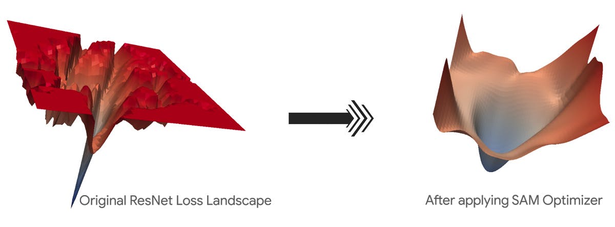
Which loss landscape do you think is easier to explore and generalizes better? ;)

Key Takeaways

Playing with hyperparameters is not the starting point for building a better model; on the contrary, tuning them is the last step, when we want to maximize learning capability and predictive accuracy of our model. Providing high quality samples, data cleaning, de-noising and feature engineering usually plays a bigger role. Also, coming up with a neural network architecture better suited for a specific task (especially if you’re into research), or utilizing SoTA models and transfer learning for your problem domain could bring in giant performance gains.

Start with the most important parameters first, because they have the most significant impacts. Undoubtedly this would require us to get to know the method and algorithm we are planning to use more in-depth; in fact, it was the approach we considered throughout this article for tuning hyperparameters of neural networks. Not all hyperparameters are actually independent, and they’re better be tuned in conjunction with relevant ones (“batch size” and “learning rate” for example, as discussed earlier). Knowing this beforehand helps a lot.

Try to keep the search space as small as possible. One way to do so is to consider few number of simultaneous parameters for tuning. Another technique is to use wisely distanced discrete values instead of large continues ranges for parameter values.

If you want to automate hyperparameter tuning and use the some great tools available out there (e.g. Optuna, Hyperopt, etc.), re-read the above takeaways. Considering them in defining the objective function and optimization steps would definitely speed things up and bring down computational cost.

Ultimately, you may find it worth trying to experiment with a hybrid approach, meaning tuning some hyperparameters manually (preferably, most impactful ones, with discrete set of values instead of continuous ranges), and some automatically. I’ve applied this procedure in several cases and it has helped for quick discoveries.

I’ll close this writing with the note that it may get occasional updates along the way. Please feel free to add anything you believe is missing, and share your thoughts and experiences in comments section.